In the previous set of lessons in this module, we learned how to train various Convolutional Neural Network (CNN) architectures, including LeNet, KarpathyNet, and MiniVGGNet, on the CIFAR-10 dataset.

Each of these networks (including even ShallowNet) were able to obtain over 50% classification accuracy, with MinIVGGNet obtaining the highest classification accuracy of 75.03%.

While we have examined how to train networks using batches of images, one aspect we have not looked at is how to take a pre-trained model and use it to classify new images — images that are not part of the original dataset.

In the remainder of this lesson, we’ll learn how to load a pre-trained network from disk and utilize it to classify and label images.

Objectives:

In this lesson, we will:

Learn how to load a pre-trained Keras model from disk.
Use our model to classify random testing images from the CIFAR-10 dataset.
Classify images that are not part of the CIFAR-10 dataset.

Running a pre-trained network

As mentioned in the introduction to this lesson, the primary goal of this tutorial is to familiarize ourselves with classifying images using a pre-trained network.

In order to accomplish this, we’ll be defining a new Python driver script named test_network.py . This script will handle:

Classifying random images from the CIFAR-10 dataset.
Taking images not part of the CIFAR-10 dataset, loading them from disk, and classifying them using our CNN.

Let’s go ahead and get started:

# import the necessary packages
from __future__ import print_function
from keras.models import load_model
from keras.datasets import cifar10
from imutils import paths
import numpy as np
import argparse
import imutils
import cv2

# construct the argument parse and parse the arguments
ap = argparse.ArgumentParser()
ap.add_argument("-m", "--model", required=True, help="path to output model file")
ap.add_argument("-t", "--test-images", required=True,
	help="path to the directory of testing images")
ap.add_argument("-b", "--batch-size", type=int, default=32,
	help="size of mini-batches passed to network")
args = vars(ap.parse_args())

We start off on Lines 2-9 by importing our required Python packages. Lines 12-18 then parse our command line arguments, which we detail below:

–model : Here we supply the path to the –model , the serialized HDF5 file that contains the weights for our network, architecture, and training state.
–test-images : This is the path to our directory of testing images.
–batch-size : The size of mini-batches to be presented to the neural network.

The next step is to select a random set of examples from the CIFAR-10 dataset:

# initialize the ground-truth labels for the CIFAR-10 dataset
gtLabels = ["airplane", "automobile", "bird", "cat", "deer", "dog", "frog", "horse",
	"ship", "truck"]

# load the network
print("[INFO] loading network architecture and weights...")
model = load_model(args["model"])

# randomly select a few testing examples from the CIFAR-10 dataset and then
# scale the data points into the range [0, 1]
print("[INFO] sampling CIFAR-10...")
(testData, testLabels) = cifar10.load_data()[1]
testData = testData.astype("float") / 255.0
np.random.seed(42)
idxs = np.random.choice(testData.shape[0], size=(15,), replace=False)
(testData, testLabels) = (testData[idxs], testLabels[idxs])
testLabels = testLabels.flatten()

Lines 21 and 22 define the set of ground-truth labels for the CIFAR-10 dataset.

Loading both our architecture and weights from disk is accomplished on Line 26 by using the load_model method of the model object.

Then, Lines 31-36 handle selecting a few testing examples at random from the CIFAR-10 dataset. We guarantee that we are using testing data by using the same pseudo-random number generator of 42 — the same value we used in training our previous networks.

We’re also sure to normalize the pixel values in the range [0, 1], just as we did during training and evaluation.

Let’s make predictions on our sample of the testing data:

# make predictions on the sample of testing data
print("[INFO] predicting on testing data...")
probs = model.predict(testData, batch_size=args["batch_size"])
predictions = probs.argmax(axis=1)

# loop over each of the testing data points
for (i, prediction) in enumerate(predictions):
	# convert the image colorspace to BGR and then enlarge it
	image = testData[i].astype(np.float32)
	image = cv2.cvtColor(image, cv2.COLOR_RGB2BGR)
	image = imutils.resize(image, width=128, inter=cv2.INTER_CUBIC)
	
	# show the image along with the predicted label
	print("[INFO] predicted: {}, actual: {}".format(gtLabels[prediction],
		gtLabels[testLabels[i]]))
	cv2.imshow("Image", image)
	cv2.waitKey(0)

Lines 40 and 41 pass the testing images through our pre-trained network, collecting the top predictions (based on the associated class label probabilities).

From there, we loop over each of the testing points (Line 44) and convert the CIFAR-10 image from a RGB image to a BGR OpenCV image.

Finally, Lines 51-54 display the output prediction to our screen.

This works great for images already part of the CIFAR-10 dataset — but what about images that are not part of CIFAR-10? How do we classify these images?

The following code block should answer these questions:

# close all open windows in preparation for the images not part of the CIFAR-10
# dataset
cv2.destroyAllWindows()
print("[INFO] testing on images NOT part of CIFAR-10")

# loop over the images not part of the CIFAR-10 dataset
for imagePath in paths.list_images(args["test_images"]):
	# load the image, resize it to a fixed 32 x 32 pixels (ignoring aspect ratio),
	# and then convert the image to RGB order to make it compatible with our network
	print("[INFO] classifying {}".format(imagePath[imagePath.rfind("/") + 1:]))
	image = cv2.imread(imagePath)
	kerasImage = cv2.resize(image, (32,32))
	kerasImage = cv2.cvtColor(kerasImage, cv2.COLOR_BGR2RGB)
	kerasImage = np.array(kerasImage, dtype="float") / 255.0

	# add an extra dimension to the image so we can pass it through the network,
	# then make a prediction on the image (normally we would make predictions on
	# an *array* of images instead one at a time)
	kerasImage = kerasImage[np.newaxis, ...]
	probs = model.predict(kerasImage, batch_size=args["batch_size"])
	prediction = probs.argmax(axis=1)[0]

	# draw the prediction on the test image and display it
	cv2.putText(image, gtLabels[prediction], (10, 35), cv2.FONT_HERSHEY_SIMPLEX,
		1.0, (0, 255, 0), 3)
	cv2.imshow("Image", image)
	cv2.waitKey(0)

On Line 62, we start looping over the images in the –test-images directory. For each of these images, we load it from disk, resize it to a fixed 32 x 32 pixels, swap color channels, and normalize each channel in the range [0, 1] (Lines 66-69).

Line 74 then constructs the kerasImage , creating a separate NumPy array with the shape (1, 32, 32, 3), which is what the Keras library expects.

Lines 75 and 76 pass the image through the network and obtain the class label prediction. The prediction is then displayed on our screen on Lines 79-82.

To classify our images using the pre-trained MiniVGGNet network, just execute the following command:

$ workon keras
$ python test_network.py --model output/cifar10_shallownet.hdf5 --test-images test_images

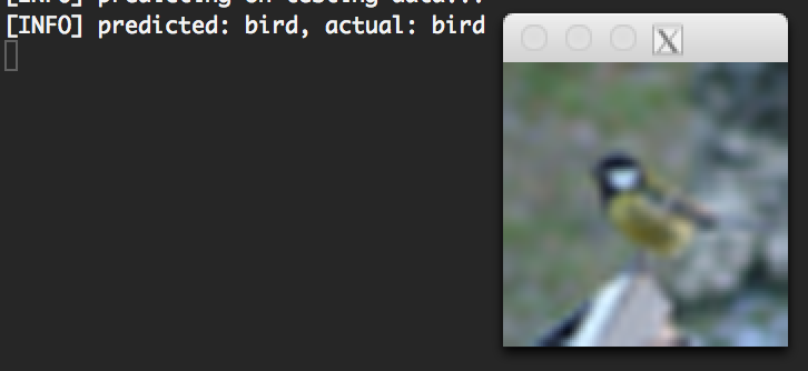
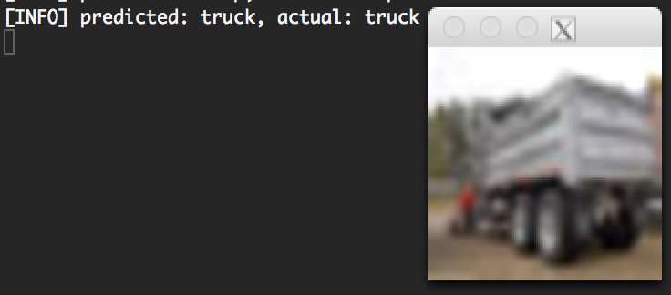
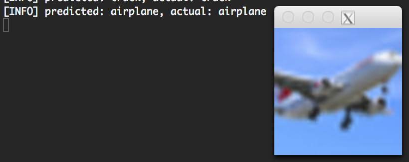
The test_network.py script first classifes a sample of testing images that are part of the CIFAR-10 dataset. The images below have been resized from their original 32 x 32 pixel size to 128 x 128 so we can more easily visualize them:

Figure 1: Classifying a "bird" using the MiniVGGNet architecture. — **Figure 1:** Classifying a “bird” using the MiniVGGNet architecture.

Figure 2: Using our trained CNN to recognize a "truck" in the image — **Figure 2:** Using our trained CNN to recognize a “truck” in the image

Figure 3: Labeling the image as "airplane". — **Figure 3:** Labeling the image as “airplane”.

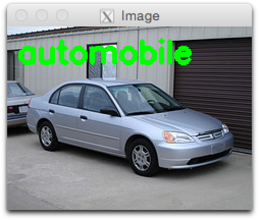
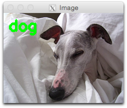
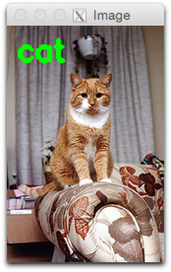
The second part of the test_network.py script takes images that are not part of the CIFAR-10 dataset. This experiment attempts to demonstrate the transfer of learning from the original dataset to images the network has never seen:

Figure 4: Our CNN is able to correctly label this image as "automobile". — **Figure 4:** Our CNN is able to correctly label this image as “automobile”.

Figure 5: MiniVGGNet has learned to recognize images from the "dog" class. — **Figure 5:** MiniVGGNet has learned to recognize images from the “dog” class.

Figure 6: Recognizing a "cat" in an image. — **Figure 6:** Recognizing a “cat” in an image.

Summary

The primary focus of this lesson has been to utilize a pre-trained network and use it to classify images that are (1) part of the CIFAR-10 dataset and (2) images that are not part of CIFAR-10.

In each case, we were able to successfully classify and label each of the images using the MiniVGGNet network. While this isn’t a “true” test of the robustness of our network, it (more importantly) demonstrates how we can serialize and load our networks from disk and utilize them to classify images that are not part of the original dataset they were trained on.

In the next set of deep learning lessons, we’ll continue this discussion of pre-trained networks — and how they can be used to alleviate the time and effort to construct new networks on a dataset-to-dataset basis.

Downloads:

Download the Code