In our previous lesson, we learned how to localize license plates in images using basic image processing techniques, such as morphological operations and contours. These license plate regions are called license plate candidates — it is our job to take these candidate regions and start the task of extracting the foreground license plate characters from the background of the license plate.
On the surface, this step looks quite easy — all we need to do is perform basic thresholding, and we’ll be able to extract the license plate characters, right?
Well, not exactly.
Sure, if we apply basic thresholding, we’ll be able to extract the license plate characters — but we’ll also extract a bunch of other “stuff” that doesn’t interest us, such as any bolts fastening the license plate to the car, branding logos on the plate itself, or embellishments on the license plate frames. All three of these aspects can cause problems for our character segmentation algorithm, so we’ll need to take special care as we write our code.
But no worries — I’ve got you covered. While there are a few “gotchas” that may trip you up, once you see them first hand, I think you’ll be able to spot them in the future when you work on your own projects.
Objectives:
In this lesson, we will:
- Apply a perspective transform to extract the license plate region from the car, obtaining a top-down, bird’s eye view more suitable for character segmentation.
- Perform a connected component analysis on the license plate region to find character-like sections of the image.
- Utilize contour properties to aide us in segmenting the foreground license plate characters from the background of the license plate.
Segmenting characters from the license plate
As a quick refresher from our previous lesson on license plate localization, our algorithm is now capable of identifying license plate-like regions in our dataset of images:
In each of the images above, you can see that we have clearly found the license plate in the image and drawn a green bounding box surrounding it.
The next step is for us to take this license plate region and apply image processing and computer vision techniques to segment the license plate characters from the license plate itself.
Character segmentation
In order to perform character segmentation, we’ll need to heavily modify our license_plate.py file from the previous lesson. This file encapsulates all the methods we need to extract license plates and license plate characters from images. The LicensePlateDetector class specifically will be doing a lot of the heavy lifting for us. Here’s a quick breakdown of the structure of the LicensePlateDetector class:
|--- LicensePlateDetector
|    |--- __init__
|    |--- detect
|    |--- detectPlates
|    |--- detectCharacterCandidates
We’ve already started to define this class in our previous lesson. The __init__ method is simply our constructor. The detect method calls all necessary sub-methods to perform the license plate detection. The aptly named detectPlates function accepts an image and detects all license plate candidates. Finally, the detectCharacterCandidates method is used to accept a license plate region and segment the license plate characters from the background.
The detectPlates function is already 100% defined from our previous lesson, so we aren’t going to focus on that method. However, we will need to modify the constructor to modify a few arguments, update the detect method to return the character candidates, and define the entire detectCharacterCandidates function.
Since we’ll be building on our previous lesson and introducing a lot of new functionality, let’s just start from the top of license_plate.py and start reworking our code:
# import the necessary packages
from collections import namedtuple
from skimage.filters import threshold_local
from skimage import segmentation
from skimage import measure
from imutils import perspective
import numpy as np
import imutils
import cv2

# define the named tupled to store the license plate
LicensePlate = namedtuple("LicensePlateRegion", ["success", "plate", "thresh", "candidates"])
The first thing you’ll notice is that we’re importing a lot more packages than from our previous lesson, mainly image processing functions from scikit-image and imutils .
We also define a namedtuple on Line 12 which is used to store information regarding the detected license plate. If you have never heard of (or used) a namedtuple before, no worries — they are simply easy-to-create, lightweight object types. If you are familiar with the C/C++ programming language, you may remember the keyword struct which is a way of defining a complex data type.
The namedtuple functionality in Python is quite similar to a struct in C. You start by creating a namespace for the tuple, in this case LicensePlateRegion , followed by a list of attributes that the namedtuple has. Since the Python language is loosely typed, there is no need to define the data types of each of the attributes. In many ways, you can mimic the functionality of a namedtuple using other built-in Python datatypes, such as dictionaries and lists; however, the namedtuple gives you a big distinct advantage — it’s dead simple to instantiate new namedtuples . In fact, as you’ll see later in this lesson, it’s as simple as passing in a list of arguments to the LicensePlate variable, just like instantiating a class!
In the meantime, the descriptions of each LicensePlate attribute are listed below:
- success : A boolean indicating whether the license plate detection and character segmentation was successful or not.
- plate : An image of the detected license plate.
- thresh : The thresholded license plate region, revealing the license plate characters on the background.
- candidates : A list of character candidates that should be passed on to our machine learning classifier for final identification.
We’ll be discussing each of these attributes in more detail as we work through the rest of this lesson, but it’s a good idea to have a high-level understanding of what we’re going to use our LicensePlate namedtuple for.
Let’s move on to our constructor:
class LicensePlateDetector:
	def __init__(self, image, minPlateW=60, minPlateH=20, numChars=7, minCharW=40):
		# store the image to detect license plates in, the minimum width and height of the
		# license plate region, the number of characters to be detected in the license plate,
		# and the minimum width of the extracted characters
		self.image = image
		self.minPlateW = minPlateW
		self.minPlateH = minPlateH
		self.numChars = numChars
		self.minCharW = minCharW
Not a whole lot has changed with our constructor, except that we are now accepting two more parameters: numChars , which is the number of characters our license plate has, and minCharW , which, as the name suggests, is the minimum number of pixels wide a region must be to be considered a license plate character.
You might be thinking, isn’t it cheating to supply a value like numChars to our LicensePlateDetector ? How do we know that the license plate we have detected contains seven characters? Couldn’t it just as easily contain five characters? Or ten?
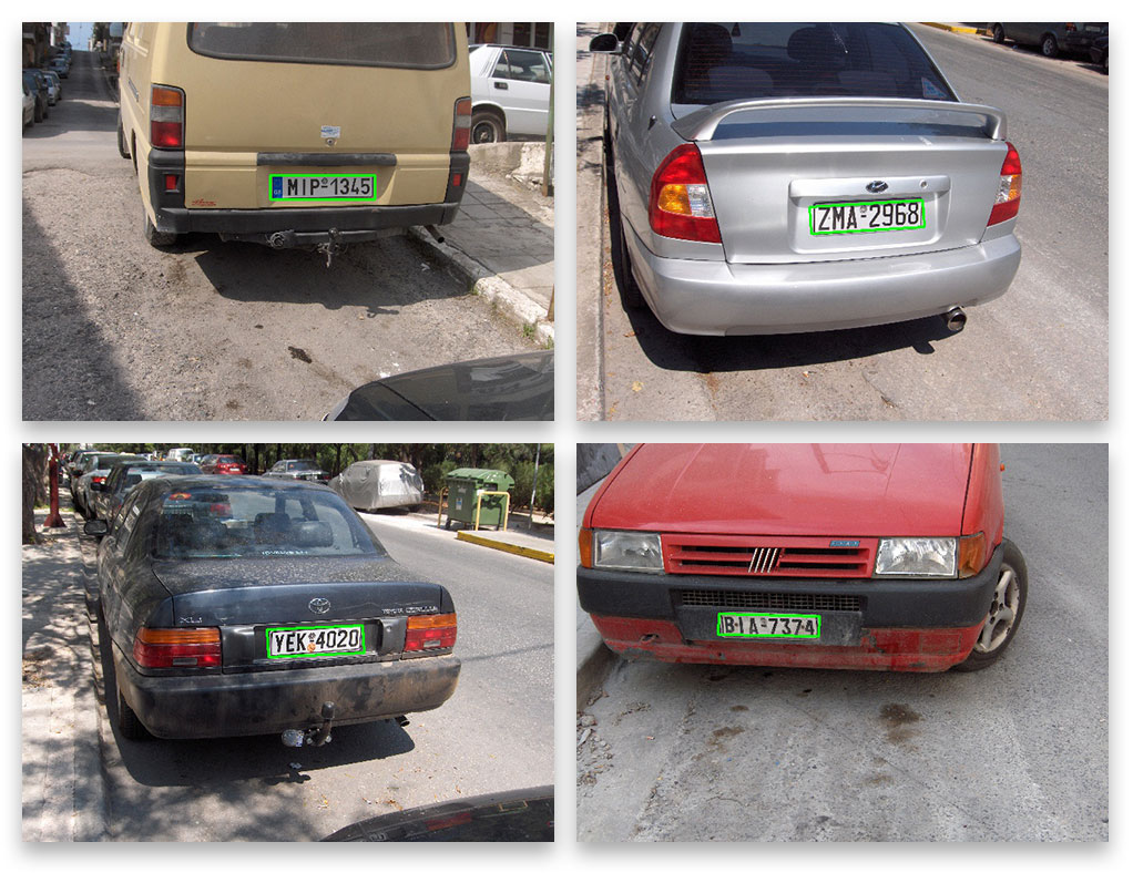
Well, as I mentioned in our What is ANPR? lesson (and is true for all computer vision projects, even ones unrelated to ANPR), we need to apply as much a priori knowledge as we possibly can to build a successful system. After examining our dataset in the previous two lessons, a clear piece of knowledge we can exploit is the number of characters present on the license plate:
In each of the above cases, all license plates contain seven characters. Thus, if we are to build an ANPR system for this region of the world, we can safely assume a license plate has seven characters. If a license plate does not contain seven characters, then we can flag the plate and manually investigate it to see (1) if there is a bug in our ANPR system, or (2) we need to create a separate ANPR system to recognize plates with a different number of characters. Remember from our introductory lesson, ANPR systems are highly tuned to the regions of the world they are deployed to — thus it is safe (and even presumable) for us to apply these types of assumptions.
Our detect method will also require a few minor updates:
	def detect(self):
		# detect license plate regions in the image
		lpRegions = self.detectPlates()

		# loop over the license plate regions
		for lpRegion in lpRegions:
			# detect character candidates in the current license plate region
			lp = self.detectCharacterCandidates(lpRegion)

			# only continue if characters were successfully detected
			if lp.success:
				# yield a tuple of the license plate object and bounding box
				yield (lp, lpRegion)
The changes here are quite self-explanatory. A call is made to detectPlates to find the license plate regions in the image. We loop over each of these license plate regions individually, make a call to the detectCharacterCandidates method (to be defined in a few short sentences), to detect the characters on the license plate region itself, and finally, return a tuple of the LicensePlate object and license plate bounding box to the calling function.
The detectPlates function is defined next, but since we have already reviewed in our license plate localization lesson, we’ll skip it in this article — please refer that lesson for the definition of detectPlates . As the name suggests, it simply detects license plate candidates in an input image.
It’s clear that all the real work is done inside the detectCharacterCandidates function. This method accepts a license plate region, applies image processing techniques, and then segments the foreground license plate characters from the background. Let’s go ahead and start defining this method:
	def detectCharacterCandidates(self, region):
		# apply a 4-point transform to extract the license plate
		plate = perspective.four_point_transform(self.image, region)
		cv2.imshow("Perspective Transform", imutils.resize(plate, width=400))
The detectCharacterCandidates method accepts only a single parameter — the region of the image that contains the license plate candidate. We know from our definition of detectPlates that the region is a rotated bounding box:
Figure 3: Our license plate detection method returns a rotated bounding box corresponding to the location of the license plate in the image.
However, looking at this license plate region, we can see that it is a bit distorted and skewed. This skewness can dramatically throw off not only our character segmentation algorithms, but also character identification algorithms when it comes to applying machine learning later in this module.
Because of this, we must first apply a perspective transform to apply a top-down, bird’s eye view of the license plate:
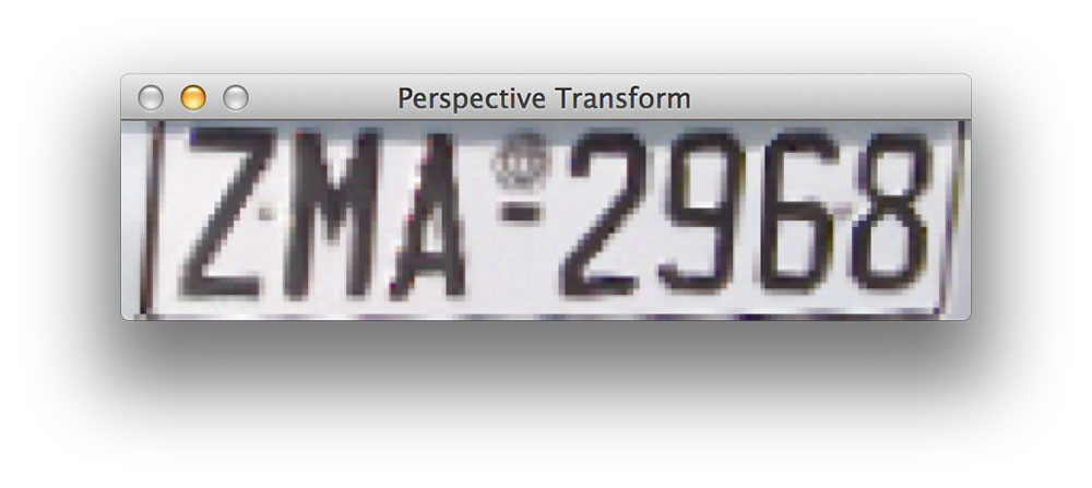
Notice how the perspective of the license plate has been adjusted, as if we had a 90-degree viewing angle, cleanly looking down on it.
Note: I cover perspective transform twice on the PyImageSearch blog. The first post covers the basics of performing a perspective transform, and the second post applies perspective transform to solve a real-world computer vision problem — building a mobile document scanner. Once we get through the first round of this course, I plan on rewriting these perspective transform articles and bringing them inside Module 1 of PyImageSearch Gurus. But for the time being, I think the explanations on the blog clearly demonstrate how a perspective transformation works.
		# extract the Value component from the HSV color space and apply adaptive thresholding
		# to reveal the characters on the license plate
		V = cv2.split(cv2.cvtColor(plate, cv2.COLOR_BGR2HSV))[2]
		T = threshold_local(V, 29, offset=15, method="gaussian")
		thresh = (V > T).astype("uint8") * 255
		thresh = cv2.bitwise_not(thresh)

		# resize the license plate region to a canonical size
		plate = imutils.resize(plate, width=400)
		thresh = imutils.resize(thresh, width=400)
		cv2.imshow("Thresh", thresh)
Now that we have a top-down, bird’s eye view of the license plate, we can start to process it. The first step is to extract the Value channel from the HSV color space on Line 109.
So why did I extract the Value channel rather than use the grayscale version of the image?
Well, if you remember back to our lesson on lighting and color spaces, you’ll recall that the grayscale version of an image is a weighted combination of the RGB channels. The Value channel, however, is given a dedicated dimension in the HSV color space. When performing thresholding to extract dark regions from a light background (or vice versa), better results can often be obtained by using the Value rather than grayscale.
To segment the license plate characters from the background, we apply adaptive thresholding on Line 110, where thresholding is applied to each local 29 x 29 pixel region of the image. As we know from our thresholding lesson, basic thresholding and Otsu’s thresholding both obtain sub-par results when segmenting license plate characters:
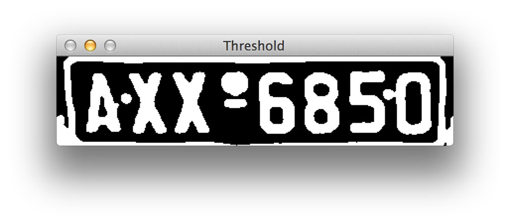
At first glance, this output doesn’t look too bad. Each character appears to be neatly segmented from the background — except for that number 0 at the end. Notice how the bolt of the license plate is attached to the character. While this artifact doesn’t seem like a big deal, failing to extract high-quality segmented representations of each license plate character can really hurt our classification performance when we go to recognize each of the characters later in this module.
Due to the limitations of basic thresholding, we instead apply adaptive thresholding, which gives us much better results:
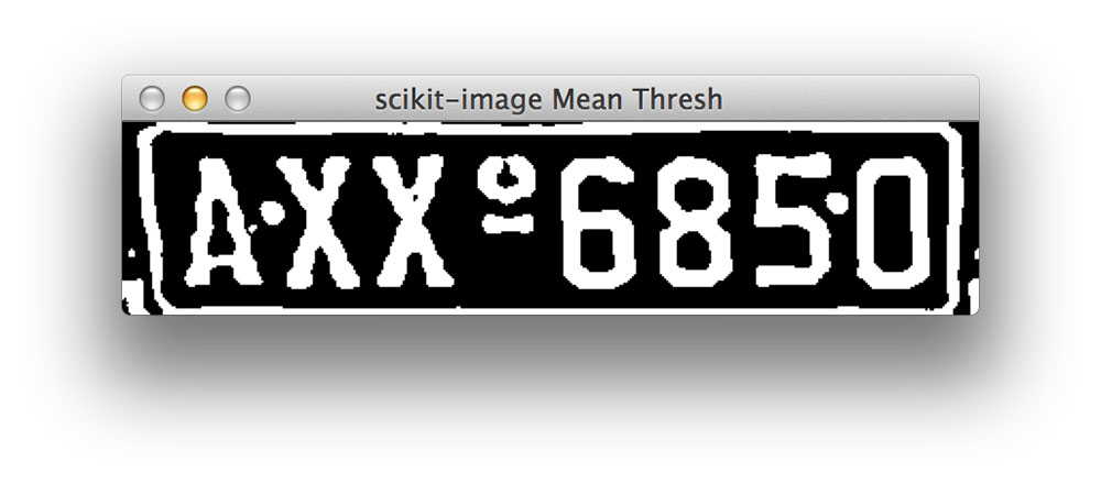
Notice how the bolt and the 0 character are cleanly detached from each other.
In previous lessons in this course, we often would apply contour detection after obtaining a binary representation of an image. However, in this case, we are going to do something a bit different — we’ll instead apply a connected component analysis of the thresholded license plate region:
		# perform a connected components analysis and initialize the mask to store the locations
		# of the character candidates
		labels = measure.label(thresh, neighbors=8, background=0)
		charCandidates = np.zeros(thresh.shape, dtype="uint8")
Given our connected component labels, we initialize a charCandidates mask to hold the contours of the character candidates on Line 122.
Now that we have the labels for each connected component, let’s loop over them individually and process them:
		# loop over the unique components
		for label in np.unique(labels):
			# if this is the background label, ignore it
			if label == 0:
				continue

			# otherwise, construct the label mask to display only connected components for the
			# current label, then find contours in the label mask
			labelMask = np.zeros(thresh.shape, dtype="uint8")
			labelMask[labels == label] = 255
			cnts = cv2.findContours(labelMask, cv2.RETR_EXTERNAL, cv2.CHAIN_APPROX_SIMPLE)
			cnts = cnts[0] if imutils.is_cv2() else cnts[1]
We start looping over each of the labels on Line 125. If the label is 0, then we know the label corresponds to the background of the license plate, so we can safely ignore it.
Note: In versions of scikit-image <= 0.11.X, the background label was originally -1. However, in newer versions of scikit-image (such as >= 0.12.X), the background label is 0. Make sure you check which version of scikit-image you are using and update the code to use the correct background label as this can affect the output of the script.
Otherwise, we allocate memory for the labelMask on Line 132 and draw all pixels with the current label value as white on a black background on Line 133. By performing this masking, we are revealing only pixels that are part of the current connected component. An example of such a labelMask can be seen below:
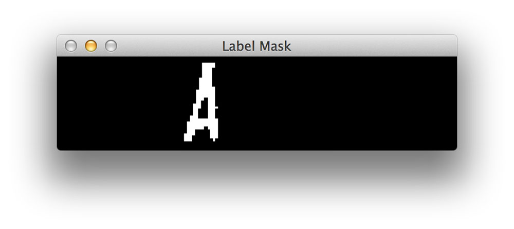
Notice how only the A character of the license plate is shown and nothing else.
Now that we have the mask drawn, we find contours in the labelMask , so we can apply contour properties to determine if the contoured region is a character candidate or not:
			# ensure at least one contour was found in the mask
			if len(cnts) > 0:
				# grab the largest contour which corresponds to the component in the mask, then
				# grab the bounding box for the contour
				c = max(cnts, key=cv2.contourArea)
				(boxX, boxY, boxW, boxH) = cv2.boundingRect(c)

				# compute the aspect ratio, solidity, and height ratio for the component
				aspectRatio = boxW / float(boxH)
				solidity = cv2.contourArea(c) / float(boxW * boxH)
				heightRatio = boxH / float(plate.shape[0])

				# determine if the aspect ratio, solidity, and height of the contour pass
				# the rules tests
				keepAspectRatio = aspectRatio < 1.0
				keepSolidity = solidity > 0.15
				keepHeight = heightRatio > 0.4 and heightRatio < 0.95

				# check to see if the component passes all the tests
				if keepAspectRatio and keepSolidity and keepHeight:
					# compute the convex hull of the contour and draw it on the character
					# candidates mask
					hull = cv2.convexHull(c)
					cv2.drawContours(charCandidates, [hull], -1, 255, -1)
First, a check is made on Line 138 to ensure that at least one contour was found in the labelMask . If so, we grab the largest contour (according to the area) and compute its bounding box.
Based on the bounding box of the largest contour, we are now ready to compute a few more contour properties. The first is the aspectRatio , or simply the ratio of the bounding box width to the bounding box height. We’ll also compute the solidity of the contour (refer to advanced contour properties for more information on solidity). Last, we’ll also compute the heightRatio , or simply the ratio of the bounding box height to the license plate height. Large values of heightRatio indicate that the height of the (potential) character is similar to the license plate itself (and thus a likely character).
You’ve heard me say it many times inside this course, but I’ll say it again — a clever use of contour properties can often beat out more advanced computer vision techniques.
The same is true for this lesson.
On Lines 151-153, we apply tests to determine if our aspect ratio, solidity, and height ratio are within acceptable bounds. We want our aspectRatio to be at most square, ideally taller rather than wide since most characters are taller than they are wide. We want our solidity to be reasonably large, otherwise we could be investigating “noise”, such as dirt, bolts, etc. on the license plate. Finally, we want our keepHeight ratio to be just the right size — license plate characters should span the majority of the height of a license plate, hence we specify a range that will catch all characters present on the license plates.
It’s important to note that these values were experimentally tuned based on our license plate dataset. For other license plate datasets these values may need to be changed — and that’s totally okay. There is no “silver bullet” for ANPR; each system is geared towards solving a very particular problem. When you go to develop your own ANPR systems, be sure to pay attention to these contour property rules. It may be the case that you need to experiment with them to determine appropriate values.
Provided that our aspect ratio, solidity, and height ratio tests pass, we take the contour, compute the convex hull (to ensure the entire bounding region of the character is included in the contour), and draw the convex hull on our charCandidates mask. Here are a few examples of computing license plate character regions:
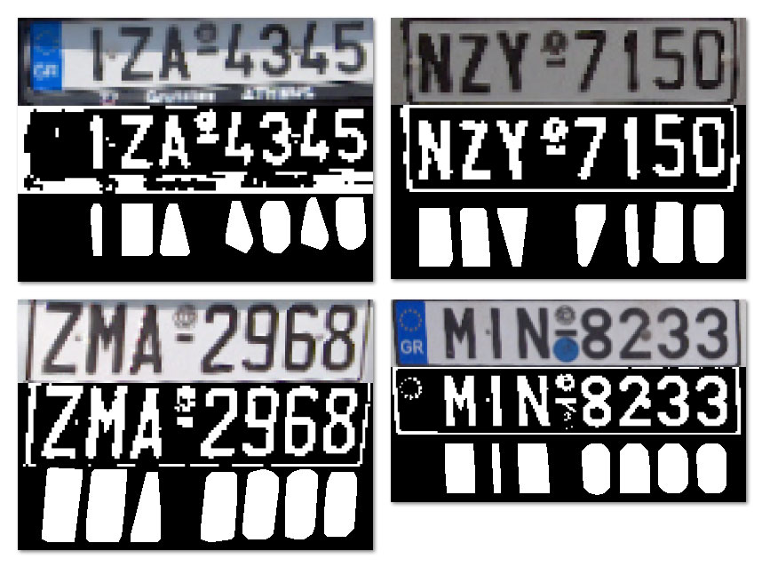
Notice in each case how the character is entirely contained within the convex hull mask — this will make it very easy for us to extract each character ROI from the license plate in the next lesson.
At this point, we’re just about done with our detectCharacterCandidates method, so let’s finish it up:
		# clear pixels that touch the borders of the character candidates mask and detect
		# contours in the candidates mask
		charCandidates = segmentation.clear_border(charCandidates)

		# TODO:
		# There will be times when we detect more than the desired number of characters --
		# it would be wise to apply a method to 'prune' the unwanted characters

		# return the license plate region object containing the license plate, the thresholded
		# license plate, and the character candidates
		return LicensePlate(success=True, plate=plate, thresh=thresh,
			candidates=charCandidates)
On Line 164, we make a call to clear_border . The clear_border function performs a connected component analysis, and any components that are “touching” the borders of the image are removed. This function is very useful in the oft case our contour property tests has a false-positive and accidentally marks a region as a character when it was really part of the license plate border.
You’ll also notice that I have placed a TODO stub on Lines 166-168. Despite our best efforts, there will still be cases when our contour property tests are just not enough and we accidentally mark regions of the license plate characters when in reality they are not. Below are a few examples of such a false classification:
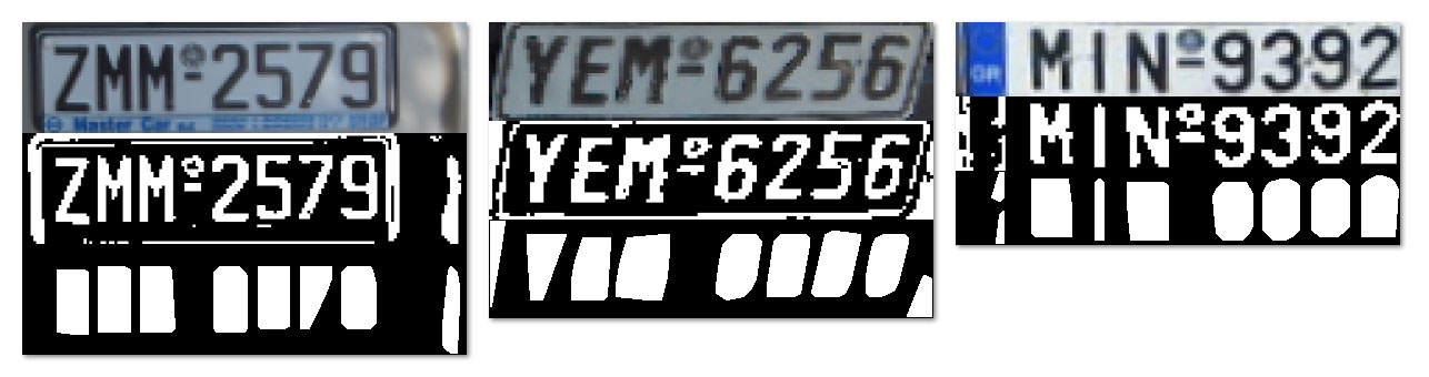
So how might we go about getting rid of these regions? The answer is to apply character pruning where we loop over the character candidates and remove the “outliers” from the group. We’ll cover the character pruning stage in our next lesson.
Remember, each and every stage of your computer vision pipeline (ANPR or not) does not have to be 100% perfect. Instead, it can make a few mistakes and let them pass through — we’ll just build in traps and mechanisms to catch these mistakes later on in the pipeline when they are (ideally) easier to identify!
Finally, we construct a LicensePlate object (Line 172) consisting of the license plate, thresholded license plate, and license plate characters and return it to the calling function.
Updating the driver script
Now that we have updated our LicensePlateDetector class, let’s also update our recognize.py driver script, so we can see our results in action:
# import the necessary packages
from __future__ import print_function
from pyimagesearch.license_plate import LicensePlateDetector
from imutils import paths
import numpy as np
import argparse
import imutils
import cv2
# construct the argument parser and parse the arguments
ap = argparse.ArgumentParser()
ap.add_argument("-i", "--images", required=True, help="path to the images to be classified")
args = vars(ap.parse_args())
# loop over the images
for imagePath in sorted(list(paths.list_images(args["images"]))):
# load the image
image = cv2.imread(imagePath)
print(imagePath)
# if the width is greater than 640 pixels, then resize the image
if image.shape[1] > 640:
image = imutils.resize(image, width=640)
# initialize the license plate detector and detect the license plates and candidates
lpd = LicensePlateDetector(image)
plates = lpd.detect()
# loop over the license plate regions
for (i, (lp, lpBox)) in enumerate(plates):
# draw the bounding box surrounding the license plate
lpBox = np.array(lpBox).reshape((-1,1,2)).astype(np.int32)
cv2.drawContours(image, [lpBox], -1, (0, 255, 0), 2)
# show the output images
candidates = np.dstack([lp.candidates] * 3)
thresh = np.dstack([lp.thresh] * 3)
output = np.vstack([lp.plate, thresh, candidates])
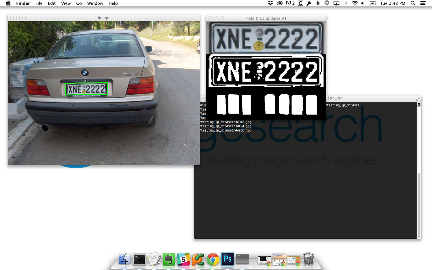
cv2.imshow("Plate & Candidates #{}".format(i + 1), output)
# display the output image
cv2.imshow("Image", image)
cv2.waitKey(0)
cv2.destroyAllWindows()
Compared to our previous lesson, not much has changed. We are still detecting the license plates on Line 27. And we are still looping over each of the license plate regions on Line 30; however, this time we are looping over a 2-tuple: the LicensePlate object (i.e. namedtuple ) and the lpBox (i.e. license plate bounding box).
For each of the license plate candidates, we construct an output image containing the (1) perspective transformed license plate region, (2) the binarized license plate region obtained using adaptive thresholding, and (3) the license plate character candidates after computing the convex hull (Lines 36-39).
To see our script in action, just execute the following command:
$ python recognize.py --images ../testing_lp_dataset
Summary
We started this lesson by building on our previous knowledge of license plate localization. We extended our license plate localizer to segment license plate characters from the license plate itself using image processing techniques, including adaptive thresholding, connected component analysis, and contour properties.
In most cases, our character segmentation algorithm worked quite well; however, there were some cases where our aspect ratio, solidity, and height ratio tests generated false positives, leaving us with falsely detected characters.
As we’ll see in our next lesson, these false positives are not as big of a deal as they may seem. Using the geometry of the license plate (i.e. the license plate characters should appear in a single row), it will actually be fairly easy for us to prune out these false positives and be left with only the actual license plate characters.
Remember, every stage of your computer vision pipeline does not have to be 100% correct every single time. Instead, it may be beneficial to pass on less-than-perfect results to the next stage of your pipeline where you can detect these problem regions and throw them away.
For example, consider the license plate localization lesson where we accidentally detected a few regions of an image that weren’t actually license plates. Instead of agonizing over these false positives and trying to make the morphological operations and contour properties work perfectly, it’s instead easier to pass them on to the next stage of our ANPR pipeline where we perform character detection. If we cannot detect characters on these license plate candidates, we just throw them out — problem solved!
Solving computer vision problems is only partially based on your knowledge of the subject — the other half comes from your creativity, and your ability to look at a problem differently and arrive at an innovative (yet simple) solution.