Unlike face detection, which is the process of simply detecting the presence of a face in an image or video stream, face recognition takes the faces detected from the localization phase and attempts to identify whom the face belongs to. Face recognition can thus be thought of as a method of person identification, which we use heavily in security and surveillance systems.

Since face recognition, by definition, requires face detection, we can think of face recognition as a two-phase process.

• Phase #1: Detect the presence of faces in an image or video stream using methods such as Haar cascades, HOG + Linear SVM, deep learning, or any other algorithm that can localize faces.
• Phase #2: Take each of the faces detected during the localization phase and identify each of them — this is where we actually assign a name to a face.

In the remainder of this lesson we’ll review a quick history of face recognition, followed by introducing the two main facial identification algorithms we’ll be covering in this module: Eigenfaces and LBPs for face recognition.

Objectives:

In this lesson we will:

• Provide a brief history of face recognition.
• Introduce the Eigenfaces and LBPs for face recognition algorithms.

What is face recognition?

Face recognition is the process of taking a face in an image and actually identifying who the face belongs to. Face recognition is thus a form of person identification.

Early face recognition systems relied on facial landmarks extracted from images, such as the relative position and size of the eyes, nose, cheekbone, and jaw. However, these systems were often highly subjective and prone to error since these quantifications of the face were manually extracted by the computer scientists and administrators running the face recognition software.

More recent face recognition systems rely on feature extraction and machine learning to train classifiers to identify faces in images. Not only are these systems non-subjective, but they are also automatic — no hand labeling of the face is required. We simply extract features from the faces, train our classifier, and then use it to identify subsequent faces.

A brief history of face recognition

In the history of computer vision, face recognition can actually be seen as a relatively “new” concept.

Prior to the work of Goldstein, et al. in the 1970’s, face recognition was often regarded as science fiction, sequestered to the movies and books set in ultra-future times. In short, face recognition was a fantasy, and whether or not it would become a reality was unclear.

This all changed in 1971 when Goldstein, et al. published Identification of human faces. A crude first attempt at face identification, this method proposed 21 subjective facial features, such as hair color and  lip thickness, to identify a face in a photograph.

The largest drawback of this approach was that the 21 measurements (besides being highly subjective) were manually computed — an obvious flaw in a computer science community that was rapidly approaching unsupervised computation and classification (at least in terms of human oversight).

Then, over a decade later in 1987, Kirby and Sirovich published their seminal work A Low-Dimensional Procedure for the Characterization of Human Faces. You may be more familiar with this work under a different name — the Eigenfaces algorithm.

Kirby and Sirovich were able to demonstrate that a standard linear algebra technique for dimensionality reduction called Principal Component Analysis  (PCA) could be used to identify a face using a feature vector smaller than 100-dim. Furthermore, the “principal components” (i.e., the eigenvectors, or the “eigenfaces”) could be used to actually reconstruct faces from the original dataset. This implies that a face could be represented (and eventually identified) as a linear combination of the eigenfaces:

Query Face = 36% of Eigenface #1 + -8% of Eigenface #2 … + 21% of Eigenface N

Following the work of Kirby and Sirovich, further research in face recognition exploded — we now see other linear algebra techniques such as Linear Discriminant Analysis being used for face recognition. These are commonly known as Fisherfaces.

Feature-based approaches such as Local Binary Patterns for face recognition have also been proposed and are still heavily used in real-world applications.

We are even starting to see deep learning applied in face identification, but normally for face alignment and funneling, a pre-processing step that takes place before the face is actually identified.

Eigenfaces

The Eigenfaces algorithm uses Principal Component Analysis to construct a low-dimensional representation of face images.

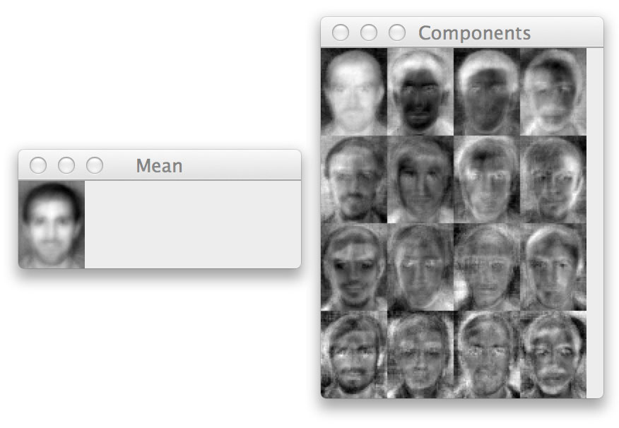
This involves collecting a dataset of faces with multiple face images per person we want to identify — like having multiple training examples of an image class we would want to label in image classification. Given this dataset of face images (presumed to be the same width, height, and ideally — with their eyes and facial structures aligned at the same (x, y)-coordinates, we apply an eigenvalue decomposition of the dataset, keeping the eigenvectors with the largest corresponding eigenvalues.

Given these eigenvectors, a face can then be represented as a linear combination of what Kirby and Sirovich call eigenfaces.

Face identification can be performed by computing the Euclidean distance between the eigenface representations and treating the face identification as a k-Nearest Neighbor classification problem — however, we tend to commonly apply more advanced machine learning algorithms to the eigenface representations.

If you’re feeling a bit overwhelmed by the linear algebra terminology or how the Eigenfaces algorithm actually works, no worries — we’ll be covering the Eigenfaces algorithm in detail in our next lesson.

LBPs for face recognition

While the Eigenfaces algorithm relies on PCA to construct a low-dimensional representation of face images, the Local Binary Patterns (LBPs) method relies, as the name suggests, on feature extraction.

First introduced by Ahonen, et al. in their 2006 paper, Face Recognition with Local Binary Patterns, their method suggests dividing a face image into an 7 x 7 grid of equally sized cells:

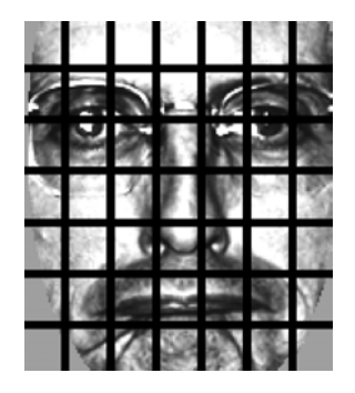
We then extract a Local Binary Pattern histogram from each of the 49 cells. By dividing the image into cells we can introduce locality into our final feature vector. Furthermore, some cells are weighted such that they contribute more to the overall representation. Cells in the corners carry less identifying facial information compared to the cells in the center of the grid (which contain eyes, nose, and lip structures). Finally, we concatenate the weighted LBP histograms from the 49 cells to form our final feature vector.

The actual face identification is performed by k-NN classification using the distance between the query image and the dataset of labeled faces — since we are comparing histograms, the distance is a better choice than the Euclidean distance.

While both Eigenfaces and LBPs for face recognition are fairly straightforward algorithms for face identification, the feature-based LBP method tends to be more resilient against noise (since it does not operate on the raw pixel intensities themselves) and will usually yield better results.

We’ll be reviewing LBPs for face recognition in detail later in this module.

Summary

In this lesson we learned that face recognition is a two-phase process consisting of (1) face detection, and (2) identification of each detected face.

We also introduced two popular algorithms for face recognition: Eigenfaces and LBPs for face recognition.

In our next lesson we’ll explore how to perform face identification using the Local Binary Patterns for face recognition algorithm.