If you’ve ever read my book, Practical Python and OpenCV + Case Studies, you’ll know that I really enjoy performing object detection/tracking using color-based methods. While it does not work in all situations, if you are able to define the object you want to track in terms of color, you can enjoy:

• A highly simplified codebase.
• Super fast object tracking that can run in super real time, easily obtaining 32+ FPS on modern hardware systems.

In the remainder of this lesson, I’ll detail an extremely simple Python script that can be used to both detect and track objects of different color in an image. We’ll start off by using two separate objects, but this same method can be extended to an arbitrary number of colored objects as well.

Objectives:

In this lesson, we will:

• Define the lower and upper boundaries of the colored objects we want to detect in the HSV color space.
• Apply the cv2.inRange  function to generate masks for each color.
• Learn how to track multiple objects of different color in webcam/video stream.

Object tracking in video

The primary goal of this lesson is to learn how to detect and track objects in video streams based primarily on their color. While defining an object in terms of color boundaries is not always possible, whether due to lighting conditions or variability of the object(s), being able to use simple color thresholding methods allows us to easily and quickly perform object tracking.

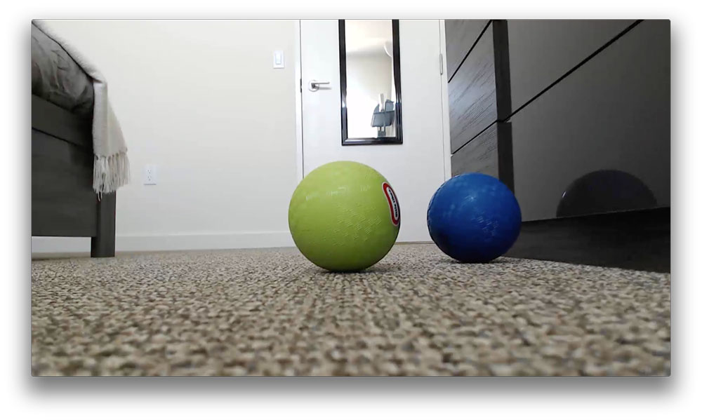
Let’s take a look at a single frame of the video file we will be processing:

As you can see, we have two balls in this image: a blue one and a green one. We’ll be writing code that can track each of these balls separately as they move around the video stream.

Let’s get coding:

# import the necessary packages
import argparse
import imutils
import cv2

# construct the argument parse and parse the arguments
ap = argparse.ArgumentParser()
ap.add_argument("-v", "--video", help="path to the (optional) video file")
args = vars(ap.parse_args())

# define the color ranges
colorRanges = [
	((29, 86, 6), (64, 255, 255), "green"),
	((57, 68, 0), (151, 255, 255), "blue")]

# if a video path was not supplied, grab the reference to the webcam
if not args.get("video", False):
	camera = cv2.VideoCapture(0)

# otherwise, grab a reference to the video file
else:
	camera = cv2.VideoCapture(args["video"])

Lines 1-9 simply handle importing our necessary packages and parsing command line arguments. We’ll accept a single, optional command line argument, –video , which is the path to the video file on disk we want to process. Otherwise, we’ll simply access the raw webcam stream of our system.

While the first few lines of our script aren’t too exciting, Lines 12-14 are especially intriguing — this is where we define the lower and upper boundaries of both the green and blue colors in the HSV color space, respectively.

A color will be considered green if the following three tests pass;

• The Hue value H is:
• The Saturation value S is:
• The Value V is:

Similarly, a color will be considered blue if:

• The Hue value H is:
• The Saturation value S is:
• The Value V is:

Obviously, the Hue value is extremely important in discriminating between these color ranges.

As a side note, whenever I teach color-based thresholding and tracking, the first question I am always asked is, “How did you know what the color ranges are for green and blue?” — I’m not going to answer that question just yet since we are in the middle of a code explanation. If you want to know the answer now, read the How did you know what these color ranges were? sub-section at the end of this lesson.

Finally, Lines 17 and 18 handle if we are accessing our webcam video stream, whereas Lines 21 and 22 will grab a pointer to our video file if a valid –video  path is indicated.

# keep looping
while True:
	# grab the current frame
	(grabbed, frame) = camera.read()

	# if we are viewing a video and we did not grab a frame, then we have
	# reached the end of the video
	if args.get("video") and not grabbed:
		break

	# resize the frame, blur it, and convert it to the HSV color space
	frame = imutils.resize(frame, width=600)
	blurred = cv2.GaussianBlur(frame, (11, 11), 0)
	hsv = cv2.cvtColor(frame, cv2.COLOR_BGR2HSV)

	# loop over the color ranges
	for (lower, upper, colorName) in colorRanges:
		# construct a mask for all colors in the current HSV range, then
		# perform a series of dilations and erosions to remove any small
		# blobs left in the mask
		mask = cv2.inRange(hsv, lower, upper)
		mask = cv2.erode(mask, None, iterations=2)
		mask = cv2.dilate(mask, None, iterations=2)

On Line 25, we start looping over each frame of our video stream. We then grab the frame  from the stream on Line 27.

We’ll process the frame a bit on Lines 35-37, first by resizing it, then by applying a Gaussian blur to allow us to focus on the actual “structures” in the frame (i.e., the colored balls), followed by converting to the HSV color space.

Line 40 starts looping over each of the individual color boundaries in the colorRanges  list.

We obtain a mask for the current color range on Line 44 by calling the cv2.inRange  function, passing in the current frame , along with the respective lower  and upper  boundaries. We then perform a series of erosions and dilations to remove any small “blobs” in the image.

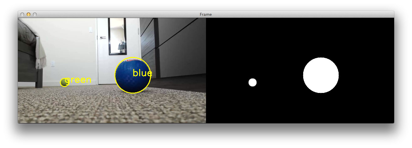
After this initial processing, our frame looks like this:

On the left, we have drawn the minimum enclosing circles surrounding each of the balls, whereas on the right, we have the clean segmentations of each ball.

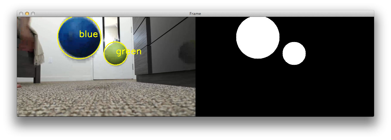
Let’s take a look at another example of ball segmentation to solidify this point:

The rest of the code in this example is quite straightforward and nothing we haven’t seen before:

		# find contours in the mask
		cnts = cv2.findContours(mask.copy(), cv2.RETR_EXTERNAL,
			cv2.CHAIN_APPROX_SIMPLE)
		cnts = cnts[0] if imutils.is_cv2() else cnts[1]

		# only proceed if at least one contour was found
		if len(cnts) > 0:
			# find the largest contour in the mask, then use it to compute
			# the minimum enclosing circle and centroid
			c = max(cnts, key=cv2.contourArea)
			((x, y), radius) = cv2.minEnclosingCircle(c)
			M = cv2.moments(c)
			(cX, cY) = (int(M["m10"] / M["m00"]), int(M["m01"] / M["m00"]))

			# only draw the enclosing circle and text if the radious meets
			# a minimum size
			if radius > 10:
				cv2.circle(frame, (int(x), int(y)), int(radius), (0, 255, 255), 2)
				cv2.putText(frame, colorName, (cX, cY), cv2.FONT_HERSHEY_SIMPLEX,
					1.0, (0, 255, 255), 2)

	# show the frame to our screen
	cv2.imshow("Frame", frame)
	key = cv2.waitKey(1) & 0xFF

	# if the 'q' key is pressed, stop the loop
	if key == ord("q"):
		break

# cleanup the camera and close any open windows
camera.release()
cv2.destroyAllWindows()

Lines 49-51 find the contours of the blob in the mask . Provided that at least one contour was found, we’ll find the largest one according to its area on Line 57.

Now that we have the largest contour of the mask, which we presume to be our ball, we compute the minimum enclosing circle, followed by the center (x, y)-coordinates of the ball (Lines 58-60). If you need a refresher on the minimum enclosing circle and centroid properties of a contour, please refer to the simple contour properties lesson of this course.

Provided that the largest contour region detected in mask  is sufficiently large, we then draw the bounding circle and the color name on the frame (Lines 64-67).

The remainder of the code simply displays the frame to our screen, handles if a key is pressed, and performs housekeeping on the video stream pointer.

Object tracking in action

Now that we have coded up our track.py  file, let’s give it a run:

$ python track.py --video BallTracking_01.mp4

We can see the output video below:

Let’s try another example, this time using a different video:

$ python track.py --video BallTracking_02.mp4

How did you know what the color ranges were?

In general, there are two methods to determine the valid color range for any color space. The first is to consult a color space chart, such as the following one for the Hue component of the HSV color space:

Based on this chart, you can define what color and shades your object falls into.

However, I dislike using this method. As we know, colors can appear dramatically different depending on our lighting conditions. Instead, I recommend a more scientific approach of gathering data, performing experiments, and validating.

Luckily, this process isn’t too challenging.

All you need to do is gather the images(s)/video of your sample objects in the desired lighting conditions, then experimentally tune the threshold values until you are able to detect only the object, ignoring the rest of the contents of the image.

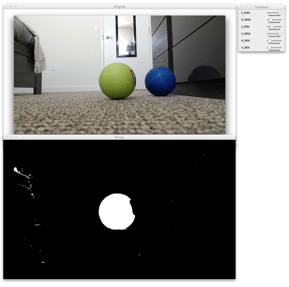
If you are using the imutils Python package, then I suggest taking a look at the range-detector script in the bin  directory. This script, created by PyImageSearch Gurus member Ahmet Sezgin Duran, can be used to determine the valid color ranges for an object using a simple GUI and sliders:

Whether you use the range-detector  script or the old-fashioned method of guess, check, and validate, determining valid color ranges will likely be a tedious, if not challenging, process at first. However, it is a task that becomes easier with practice.

Summary

In this lesson, we learned how to track objects (specifically balls) in a video stream based on their color. While it is not always possible to detect and track an object based on its color, it does yield two significant benefits, including (1) a small, simple codebase and (2) extremely speedy and efficient tracking, obtaining super real time performance.

The real trick when tracking an object based on only its color is to determine the valid ranges for the given shade. I suggest using the HSV or L*a*b* color space when defining these ranges as they are much more intuitive and representative of how humans see and perceive color. The RGB color space is often not a great choice, unless you are working under very tightly controlled lighting conditions or you only have to track one object rather than multiple.

Determining the appropriate color range for a given object can be accomplished either experimentally (i.e., guessing, checking, and adapting) or by using a tool such as the range-detector  in the imutils package.

Downloads:

Download the Code